4 minutes
Climate map using leaflet
The following tutorial explains how to generate an interactive map employing the R-library: leaflet.
library(leaflet)
library(geojsonio) # required to read json file
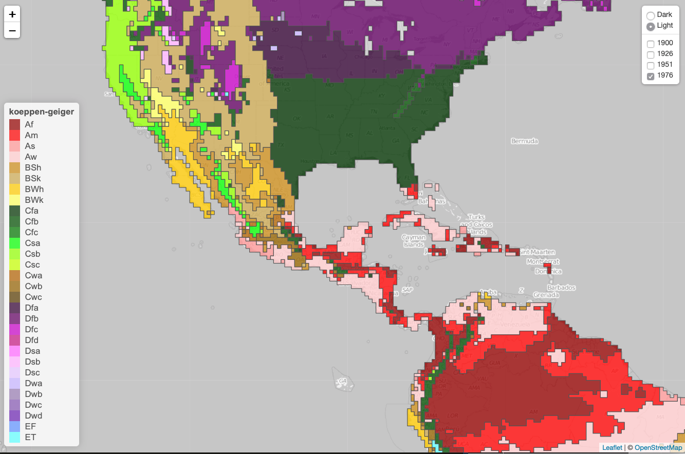
library(leaflet.extras) # simplifies addition of featuresThe following example displays the Köppen-Geiger climate classification map1, which categorises world regions based on observed temperature and precipitation conditions. In the study1, a set of underlying data regarding both observed and projected climates shifts is made freely available2. This example only utilises the observed conditions for four different periods: 1900-1925, 1926-1950, 1951-1975, 1976-2000. Each of these files with observed conditions contains lines of grid box centre coordinates (latitude, longitude), with their corresponding climate class.
To simplify the processing of information, the example employs a set of processed topo-json files 3, as well as a json file outlining the countries of the world 4.
Hands-on
First, a table of colours is loaded, whose values are those defined in the aforementioned study 1.
tblColors <- read.table("myData/koeppen/koeppen_lgd.txt", header = TRUE, stringsAsFactors = F)Now, these datasets contain the class for each polygon/square, but do not contain the preferred colour. This can be achieved in two ways: 1) by comparing the class with the table of colours when the leaflet object is called, or 2) by assigning the colour to the class in the dataset. The later is expectedly faster, and the process is developed in the function fnAddFeatures.
fnAddFeatures <- function(dtaJson, dtaPal=tblColors){

  dtaJson$style = list(
    weight = 1,
    color = "#555555",
    opacity = 1,
    fillOpacity = 0.8
  )

  geometries <- sapply(dtaJson$features, function(feat) {
    feat$properties$gridcode}
  )

  dtaJson$features <- lapply(dtaJson$features, function(feat){
    feat$properties$style <- list(
      fillColor = dtaPal$col[dtaPal$class %in% feat$properties$gridcode]
    )
    feat

  })

  return(dtaJson)
}
The function fnAddFeatures adds a general style attribute. It then extracts the gridcode class, and stores it in the object geometries. Finally, a new feature called style compares the gridcode with the table of colours for each element of the list—therefore the use of lapply.
Now the four datasets are loaded, and the style feature is added.
Clim1900 <- fnAddFeatures(geojson_read(paste(path.Project,"myData/ClimateMap/climate-map-master/1901-1925.topo.json",sep="/")))
Clim1926 <- fnAddFeatures(geojson_read(paste(path.Project,"myData/ClimateMap/climate-map-master/1926-1950.topo.json",sep="/")))
Clim1951 <- fnAddFeatures(geojson_read(paste(path.Project,"myData/ClimateMap/climate-map-master/1951-1975.topo.json",sep="/")))
Clim1976 <- fnAddFeatures(geojson_read(paste(path.Project,"myData/ClimateMap/climate-map-master/1976-2000.topo.json",sep="/")))
The map
A random location is defined for the setview, and the extent to which the map can be zoomed-out is defined.
setView(lng = -105, lat = 23, zoom = 3) %>%

setMaxBounds(lng1 = -178.5241, lat1 = -72.05115,
             lng2 = 178.52414, lat2 = 65.05115 ) %>%
Two base maps are defined here: light and dark, which can be selected in the control panel.
addProviderTiles("CartoDB.DarkMatterNoLabels",
                 options = providerTileOptions(minZoom = 2, maxZoom = 7),
                 group = "Dark") %>%
addProviderTiles("OpenStreetMap.BlackAndWhite",
                 options = providerTileOptions(minZoom = 2, maxZoom = 7, noWrap = TRUE),
                 group = "Light") %>%
addLayersControl(baseGroups = c("Dark", "Light"),
                 options = layersControlOptions(collapsed = FALSE))
Each dataset is aded to a addGeoJSON object, and a group is assigned to be included in the control menu/legend.
addGeoJSON(Clim1900, weight = 0.4, group = "1900") %>% hideGroup("1900") %>%
addGeoJSON(Clim1926, weight = 0.4, group = "1926") %>% hideGroup("1926") %>%
addGeoJSON(Clim1951, weight = 0.4, group = "1951") %>% hideGroup("1951") %>%
addGeoJSON(Clim1976, weight = 0.4, group = "1976") %>% hideGroup("1976") %>%
addGeoJSONv2(World, color = "white", weight = 0.6, popupProperty = "popup", labelProperty = "ADMIN") %>%

addLegend(position = "bottomleft", colors = tblColors$col,
          labels = tblColors$class, opacity = 0.75,
          labFormat = labelFormat(
            prefix = "(", suffix = ")%", between = ", "),
          title = "koeppen-geiger") %>%
The following action wraps up the definition of the leaflet object.
m <- leaflet() %>%
  setView(lng = -105, lat = 23, zoom = 3) %>%
  addProviderTiles("CartoDB.DarkMatterNoLabels",
                   options = providerTileOptions(minZoom = 2, maxZoom = 7),
                   group = "Dark") %>%
  addProviderTiles("OpenStreetMap.BlackAndWhite",
                   options = providerTileOptions(minZoom = 2, maxZoom = 7, noWrap = TRUE),
                   group = "Light") %>%
  setMaxBounds( lng1 = -178.5241, lat1 = -72.05115,
                lng2 = 178.52414, lat2 = 65.05115 ) %>%
  addLegend(position = "bottomleft", colors = tblColors$col,
            labels = tblColors$class, opacity = 0.75,
            labFormat = labelFormat(
              prefix = "(", suffix = ")%", between = ", "),
            title = "koeppen-geiger") %>%
  addGeoJSON(Clim1900, weight = 0.4, group = "1900") %>% hideGroup("1900") %>%
  addGeoJSON(Clim1926, weight = 0.4, group = "1926") %>% hideGroup("1926") %>%
  addGeoJSON(Clim1951, weight = 0.4, group = "1951") %>% hideGroup("1951") %>%
  addGeoJSON(Clim1976, weight = 0.4, group = "1976") %>% hideGroup("1976") %>%
  addGeoJSONv2(World, color = "white", weight = 0.6, popupProperty = "popup", labelProperty = "ADMIN") %>%
  addLayersControl(overlayGroups = c("1900", "1926", "1951", "1976"),
                   baseGroups = c("Dark", "Light"),
                   options = layersControlOptions(collapsed = FALSE))

m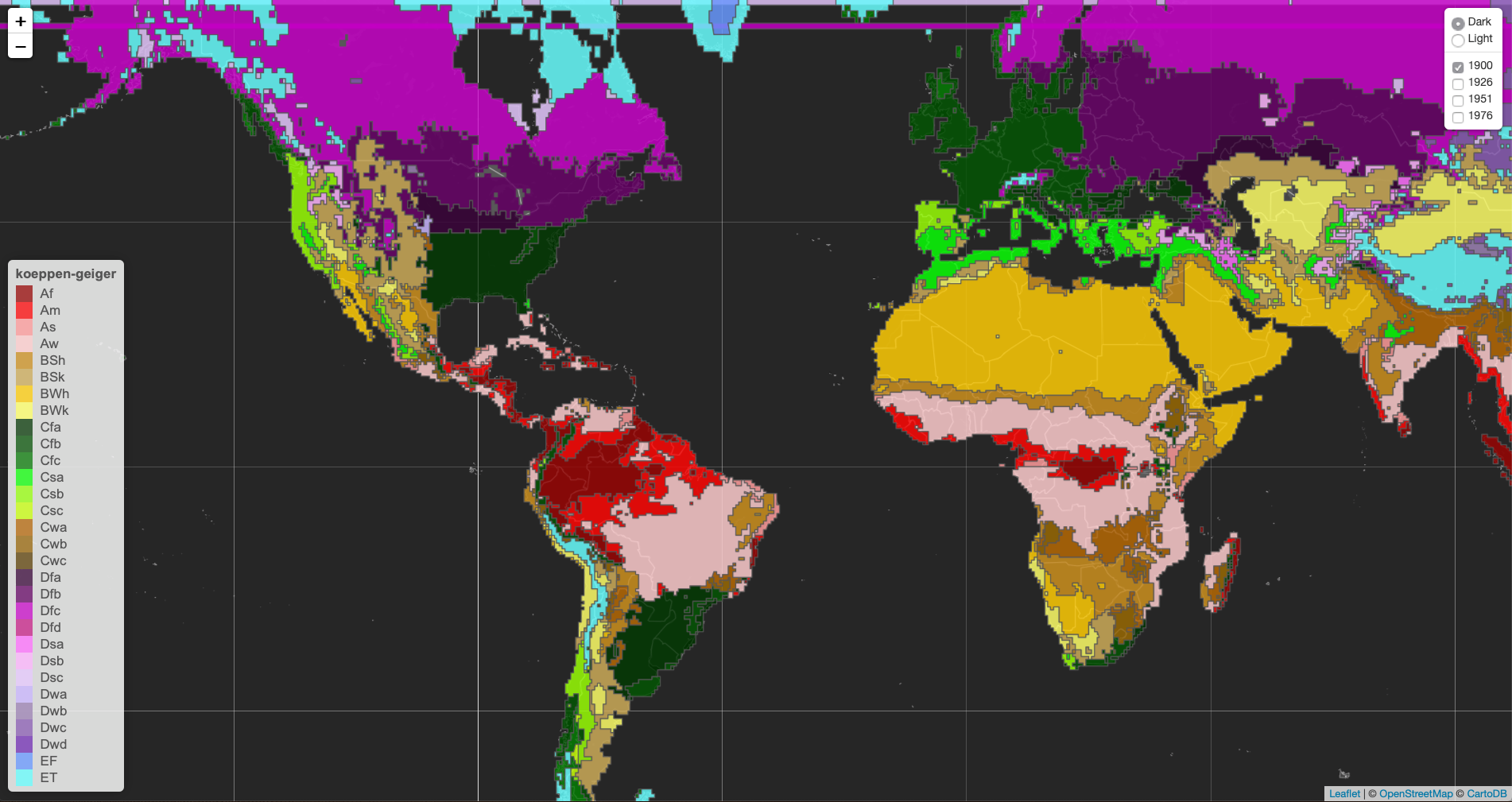
One last thing, how about a different projection?
crs.molvidde <- leafletCRS(
  crsClass="L.Proj.CRS", code='ESRI:53009',
  proj4def= '+proj=moll +lon_0=0 +x_0=0 +y_0=0 +a=6371000 +b=6371000 +units=m +no_defs',
  resolutions = c(65536, 32768, 16384, 8192, 4096, 2048))

leaflet(options = leafletOptions(maxZoom = 2,
crs= crs.molvidde, attributionControl = FALSE)) %>% 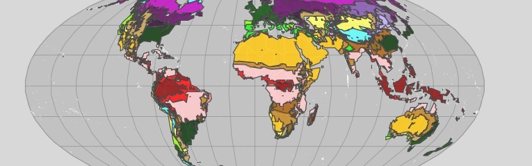
I hope this has been useful.
[- Download table of colours]
.
Maps ©OpenStreetMap contributors unless otherwise noted.
- Rubel, F., and M. Kottek, 2010: Observed and projected climate shifts 1901-2100 depicted by world maps of the Köppen-Geiger climate classification. Meteorol. Z., 19, 135-141. DOI: 10.1127⁄0941-2948/2010/0430. [return]
- http://koeppen-geiger.vu-wien.ac.at/shifts.htm [return]
- https://github.com/circleofconfusion/climate-map [return]
- Country Polygons as GeoJSON, in http://datahub.io [return]